Model data and settings

Energy demand sectors

The energy demand sectors included the industry, buildings, and transport sectors, which are further disaggregated into several subsectors as below. Details on the energy end-use representations are summarized in the following sections. Energy consumption in 2010, which is the base year in AIM/Technology-Japan, is calibrated based on the World Energy Balances of the International Energy Agency [1]. Japan’s national energy balance table [2] is also used to calibrate sectoral energy demands.

Sector and service disaggregation of the energy demand sectors.

Sector	Subsector	Service and mode
Industry	Steel, cement, petrochemical, pulp and paper, non-ferrous metals, other non-metallic minerals, other chemical products, machinery, textile, food, other products, construction, agriculture, forestry and fisheries	-
Buildings	Residential, commercial	Air conditioning, water heating, cooking, lighting, other appliances
Transport	Passenger, freight	Road, rail, domestic navigation, domestic aviation

Industry

AIM/Technology-Japan includes the following industrial subsectors: steel, cement, petrochemical, pulp and paper, non-ferrous metals, other non-metallic minerals, other chemical products, machinery, textile, food, other products, construction, and agriculture, forestry and fisheries. In the steel, cement, petrochemical, and pulp and paper sectors, sector-specific energy technologies are considered, based on the literature [3] [4] [5], whereas the other sectors are assumed to employ common technologies such as the boiler, furnace, and motor. The technological parameter assumption is summarized in the appendix. Introduction of CCS is assumed in the steel and cement sectors. Most energy consumption for non-energy use is assumed to be related to the industrial sector.

Buildings

The buildings sector is disaggregated into residential and commercial sectors, and energy devices are explicitly modeled for each subsector, including air conditioning, water heating, cooking, lighting, and other appliances. Energy consumption in the base year for various energy service types and technical parameters is estimated based on previous studies [4] [5] [6]. The technological parameter assumption is summarized in the appendix. The technology list included energy-efficient building devices and fuel changes from fossil fuels to low-carbon carriers such as electricity and hydrogen. Energy efficiency improvement in building envelopes is also considered.

Transportation

The transport sector covered both passenger and freight transport in four modes, namely road, rail, marine navigation, and aviation. In addition, road transport is disaggregated in terms of vehicle size into large and small vehicles, as well as buses for passenger transport. In each subsector and mode, improved fuel economy is considered the mitigation option. For road transport, the fuel switch from fossil fuels to low-carbon carriers, such as electricity and hydrogen, is also taken into account. The technological parameter assumption is summarized in the appendix. International bunkers are not included in AIM/Technology-Japan.

Energy supply sectors and others

Energy conversion

AIM/Technology-Japan V2.1 contains a detailed power sector module, as documented by Oshiro et al. [7]. This module considers the balance of electricity supply and demand with 1-hour temporal resolution to determine the impact of variable renewable energies (VREs). The model generates specific electricity demand hourly curves for several representative load profiles, including four representative days in summer, winter, and intermediate seasons, where demand peak day is explicitly represented. The hourly electricity demand profile for the simulation years for each region is generally assumed to be identical to that of the base year, whereas the effect of demand response on the demand profile is explicitly modeled. In AIM/Technology-Japan, electric heat pump water heaters in the buildings sector, battery electric vehicles, and electrolysis can act as demand response resources, as their operating hours can be changed to provide flexibility. In addition, electricity storage can also contribute to balancing hourly electricity demand and supply. In this model, pumped hydro storage and batteries are considered storage technologies. Inter-seasonal storage is not considered.

VREs, including solar photovoltaic, wind, and ocean power, require backup capacity with flexible power resources due to their intermittency. The hourly power generation profile is based on the Renewables.ninja [8] [9]. Interregional transmission capacity is explicitly modelled. Power generation costs are estimated based on the literature [10] [11]. The parameter assumptions in this model are summarized in the appendix.

As hydrogen-based energy carriers, hydrogen, ammonia and synfuel production, based on electrolysis, coal, natural gas and biomass, is modelled. Their production efficiency and cost are taken from IEA literature [12], as summarized in the appendix.

CO2 emissions from synfuel combustions are accounted in the production phase of synfuels. Biomass to liquids parameters are based on GEA [13].

Primary energy supply

As most fossil fuels used in Japan are imported, the primary energy prices of fossil fuels need to be provided as exogenously scenarios, which are estimated by AIM/Technology-Global or based on the International Energy Agency outlook [14] [15]. The typical assumptions of fossil fuel primary energy prices taken from AIM/Technology-Global are summarized below. No fossil reserve constraints are considered in the model.

Assumptions on fossil fuel primary energy prices (Unit: US$ GJ ^-1)

	2010	2020	2030	2040	2050
Coal	4.1	4.6	4.6	4.6	5.1
National gas	9.9	10.2	9.7	9.7	9.7
Crude oil	12.8	10.4	11.9	12.6	13.6

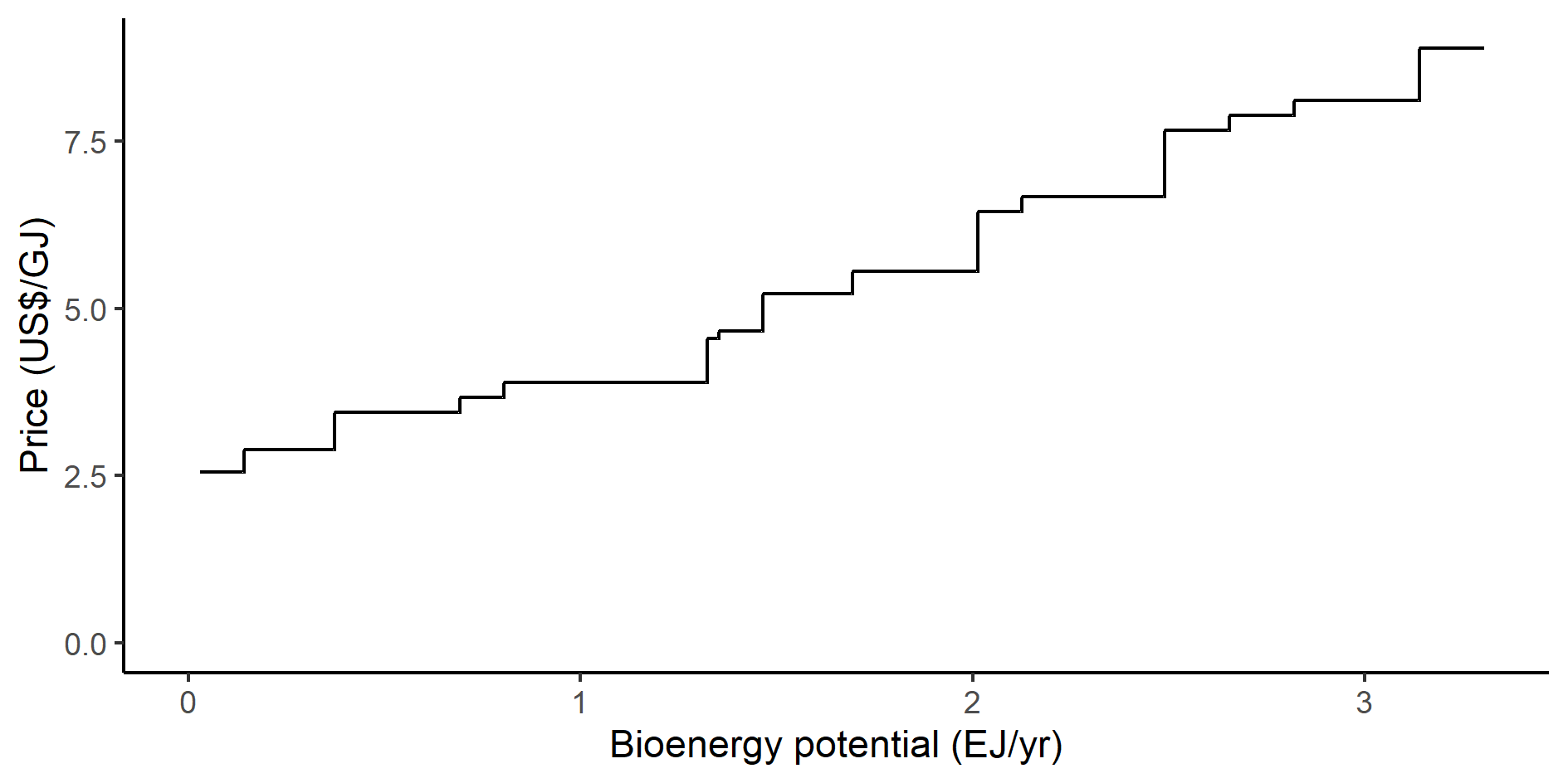
Renewable energy potentials are obtained from a survey released by the Ministry of Environment [16] [17]. Rooftop PV has four capacity factor grade, ranging from 12% to 16%, based on the grid data taken from MOE [17]. Biomass potential and production cost curve are shown below, which are based on Wu, et al. [18], with four cost grades for surplus woods, forestry residues, livestock residues, municipal solid wastes, dedicated energy crops and black liquors.

Supply cost curve of bioenergy, including surplus woods, forestry residues, livestock residues, municipal solid wastes, and dedicated energy crops.

Unless otherwise noted (e.g. No-Nuclear scenario), the maximum capacity and generation from nuclear power plant is set to be consistent with the NDC assumptions in Japan, which are documented by Oshiro, et al. [19], where the maximum power generation from nuclear power is given based on the New Policies Scenario of the World Energy Outlook 2014 [20] which assumed the extension of the lifetime of nuclear plants build since the mid-1980s up to 60 years. Based on these assumptions, maximum power generation from nuclear power in 2030 accounts for approximately 232 TWh, which is coherent with the assumptions of the NDC (217-232 TWh in 2030).

Carbon storage and utilization

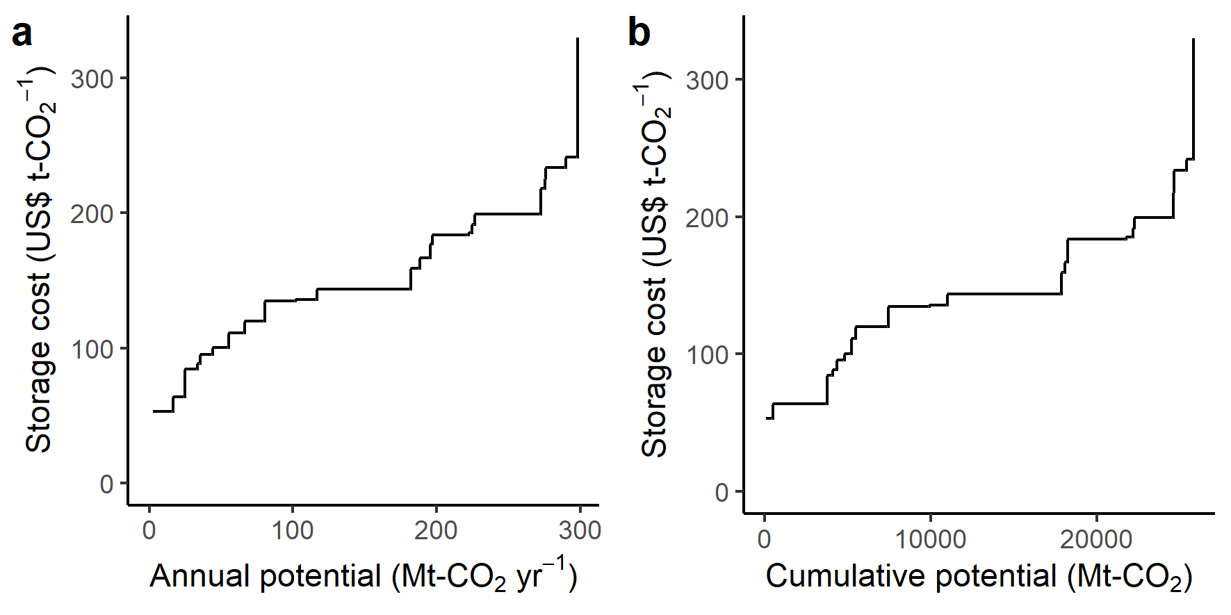
Constraints for both annual and cumulative storage potential are imposed in AIM/Technology-Japan. For the storage sites, aquifer and enhanced oil recovery (EOR) are assumed. Underground storage potential and cost are estimated based on RITE as summarized in [21] [22] .

Carbon utilization for energy and feedstock is considered. In the energy sector, liquid fuels (gasoline, kerosene, diesel and jet fuels) and gases can be replaced by synthetic liquids and methanation, respectively. For feedstock use, petrochemical goods are assumed to be converted from synthetic hydrocarbon. CO₂emissions associated with synthetic hydrocarbon are accounted in the production process, namely in the hydrogen generation sector rather than the end-use sectors. Conversion efficiency and cost parameters associated with carbon utilization are summarized in appendix.

As a carbon capture option, direct air capture (DAC) is also considered as negative emission technology as well as fossil fuels, industrial processes and BECCS, whose parameter assumptions are based on Realmonte, et al. [23] as below.

Parameter assumptions for direct air capture

Capital cost (US$ kg-CO2-1)	1.146
O&M cost (US$ kg-CO2-1)	0.042
Electricity demand (MJ kg-CO2-1)	1.3
Heat demand (MJ kg-CO2-1)	5.3
Capture rate	95%

Storage cost curve for CO₂underground storage for a) annual storage potential and b) cumulative storage potential.

Other sectors

AIM/Technology-Japan covers non-energy sectors as well. The parameters on mitigation measures are based on the literatures [24] [25].

Socio-economic parameters

Energy service demand, including industrial production and transport demand, must be input into AIM/Technology-Japan. Details regarding energy service demand estimation are also documented in Oshiro et al. [26] .

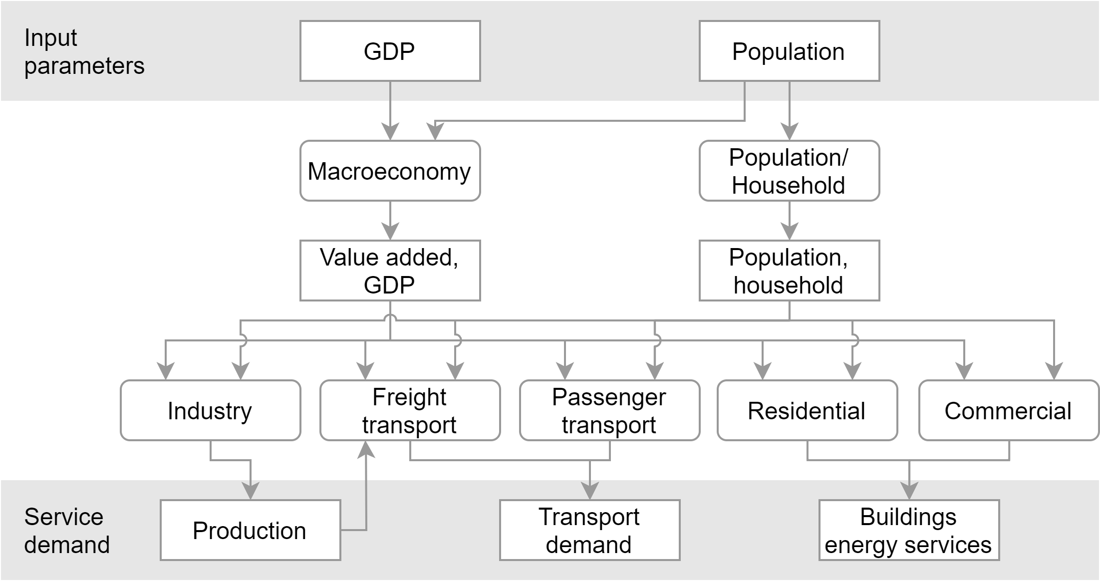
Schematic overview of the energy service demand model. Indicators are displayed in rectangles, and models and modules are displayed in rounded rectangles.

Gross domestic product (GDP) and population are the basic input parameters for the energy service demand model. First, the sectoral value-added and number of households are estimated with the macroeconomy and population/household modules, respectively. Second, sectoral energy service demands are estimated based on the sectoral modules. The following subsections describe the details of each submodule.

Macroeconomy

Macroeconomic indicators are estimated based on [27]. The GDP is split according to the sectoral value added for the agricultural, industrial, and service sectors based on a multi-nominal logit function with GDP per capita as an explanatory variable. Sectoral value added is estimated using equations below.

\[{VA}_{se} = GDP\cdot {RVA}_{se}\]

\[{RVA}_{AGR} = \left(1+{LRVA}_{IND}+{LRVA}_{IND}\cdot {LRVA}_{SER}\right)^{-1}\]

\[{RVA}_{IND} = {LRVA}_{IND}\cdot {RVA}_{AGR}\]

\[{RVA}_{SER} = {LRVA}_{SER}\cdot {RVA}_{IND}\]

Formula	\(a_0\)	\(a_1\)	\(R^2\)
\(\ln⁡{LRVA}_{IND} = a_0+a_1\cdot \ln \frac{GDP}{POP}\)	1.17*** (14.71)	1.35*** (20.54)	0.92
\(\ln{LRVA}_{SER} = a_0+a_1\cdot \ln \frac{GDP}{POP}\)	0.63*** (13.93)	0.30*** (7.96)	0.62

Note: Numbers in parenthesis indicates t-value. Asterisks indicate p-value ranges at \(p \le 0.001 (***)\), \(p \le 0.01 (**)\), \(p \le 0.05 (*)\), \(p \le 0.1 ( )\)

Symbol	Description
\({VA}_{se}\)	Value added in economic sector se. \(se = \{AGR,SER,IND\}\)
\(GDP\)	Gross domestic product
\(POP\)	Population
\({RVA}_{se}\)	Share of sectoral value in GDP
\({LRVA}_{IND}\)	Ratio of \({RVA}_{IND}\) to \({RVA}_{AGR}\)
\({LRVA}_{SER}\)	Ratio of \({RVA}_{SER}\) to \({RVA}_{IND}\)

where \(AGR\), agriculture; \(SER\), service; \(IND\), industry.

Population and households

Population and household predictions are based on the AIM/PHM (Population and Household Model) [5]. The equations of AIM/PHM are summarized in equations below. When the population estimation is provided exogenously (e.g. using Shared Socio-economic Pathways), only the households related equation is used. The parameters are taken from the reports of the National Institute of Population and Social Security Research [28].

\[{POP}_{r,s,y,t+1} = {POP}_{r,s,y,t}+{BIR}_{r,s,y,t}-{MOR}_{r,s,y,t}+{MIG}_{r,s,y,t}\]

\[{BIR}_{r,s,y,t+1} = {POP}_{r,s,y,t}\cdot {br}_{r,s,y,t}\]

\[{MOR}_{r,s,y,t+1} = {POP}_{r,s,y,t}\cdot \left(1-{sr}_{r,s,y,t}\right)\]

\[{MIG}_{r,s,y,t+1} = {POP}_{r,s,y,t}\cdot {mg}_{r,s,y,t}\]

\[H_{r,t+1} = \sum_{s,y}\left({POP}_{r,s,y,t}\cdot {hh}_{r,s,y,t}\right)\]

Symbol	Description
\({POP}_{r,s,y,t}\)	population in region \(r\) with sex \(s\) and age \(y\) in year \(t\).
\({BIR}_{r,s,y,t}\)	births
\({MOR}_{r,s,y,t}\)	mortality
\({MIG}_{r,s,y,t}\)	migration
\(H_{r,t}\)	number of households
\({br}_{r,s,y,t}\)	birth rate
\({sr}_{r,s,y,t}\)	survival rate
\({mg}_{r,s,y,t}\)	migration rate
\({hh}_{r,s,y,t}\)	ratio of households to population

Industry

Industrial service demand is represented as material production or indices of industrial production in AIM/Technology-Japan, which are generally estimated through regression analysis based on historical time-series data. The industrial sector in AIM/Technology-Japan includes the following subsectors: steel, cement, petrochemical, pulp and paper, non-ferrous metals, other non-metallic minerals, other chemicals, machinery, textile, food, other products, construction, and agriculture, forestry, and fisheries.

Steel production is estimated based on the global steel demand and production model, as steel is a global commodity and therefore cannot be estimated using only internal economic drivers. The steel production model is based on that of Akashi, et al. [27]. Other industrial production levels are estimated using a regression model based on historical time-series data.

Steel

As steel products are a global commodity and future national production cannot be readily explained based solely on Japan’s domestic socio-economic conditions, we employed a global steel demand and production model. A detailed description of the global steel model has been published previously [27]. The domestic and international market equilibrium equations are presented as the following equations.

\[{CNS}_r = {PRD}_r - {EXC}_r + {MC}_r\]

\[\sum_r{EXC}_r = \sum_r{MC}_r\]

Other industries

Production levels and production indices in other industrial sectors are estimated using the regression model. For non-ferrous metal estimation, a dummy variable is used before 1981, as the statistical method is changed after 1982. The data used for estimation are time-series data taken from the literature [6].

Symbol	Description
\({PROD}_{si}\)	Industrial production in industrial subsector \(si\)
\({IIP}_{si}\)	Index of industrial production in industrial subsector \(si\)
\(T\)	Time trend (1951 = 1)
\(D_{81}\)	Dummy variable for 1981 or before

Summary of regression model for industrial production estimation.

Sector	Formula	\(a_0\)	\(a_1\)	\(a_2\)	\(a_3\)	\(R^2\)
Cement	\(\ln{PROD}_{cement} = a_0+a_1\cdot\ln⁡{VA}_{IND}+a_2\cdot\ln{T}\)	-0.34 (-0.23)	1.42*** (8.43)	-1.27*** (-9.19)		0.69
Paper	\(\ln{PROD}_{paper} = a_0+a_1\cdot\ln\frac{GDP}{POP}+a_2\cdot\ln⁡{POP}_{15-64}\)	-10.8*** (-4.07)	0.76*** (16.1)	1.77*** (7.44)		0.97
Petrochemical	\(\ln{PROD}_{ethylene} = a_0+a_1\cdot\ln{IIP}_{Chemical}+a_2\cdot\ln{T}\)	5.03*** (25.1)	1.22*** (9.72)	-0.44** (-3.34)		0.90
Other chemicals	\(\ln{IIP}_{chemical} = a_0+a_1\cdot\ln\frac{GDP}{POP}+a_2\cdot\ln{POP}+a_3\cdot\ln⁡{T}\)	-42.37*** (-6.19)	1.07*** (9.72)	3.95*** (6.67)	-0.22*** (-4.4)	0.99
Minerals	\(\ln⁡{IIP}_{mineral} = a_0+a_1\cdot\ln{VA}_{IND}+a_2\cdot\ln{T}\)	-3.70*** (-7.68)	1.20*** (22.9)	-1.40*** (-35.5)		0.98
Non-ferrous metals	\(\ln⁡{IIP}_{metal} = a_0+a_1\cdot\ln⁡{VA}_{IND}+a_2\cdot\ln⁡{D_{81}}\)	-3.70** (-3.54)	0.71*** (7.83)	0.31*** (4.38)		0.64
Machinery	\(\ln{IIP}_{machine} = a_0+a_1\cdot\ln⁡{GDP}\)	-7.12*** (-10.7)	0.89*** (17.4)			0.89
Food	\(\ln⁡{IIP}_{food} = a_0+a_1\cdot\ln⁡\frac{GDP}{POP}+a_2\cdot\ln{POP}+a_3\cdot\ln{T}\)	-19.07*** (-4.21)	0.38*** (5.26)	2.16*** (5.52)	-0.54*** (-16.4)	0.90
Chemical textiles	\(\ln⁡{IIP}_{textile} = a_0+a_1\cdot\ln⁡{VA}_{IND}+a_2\cdot\ln{T}\)	-3.10 (-1.99)	1.39*** (8.21)	-2.08*** (-16.3)		0.92
Other industries	\(\ln⁡{IIP}_{other} = a_0+a_1\cdot\ln⁡{VA}_{IND}+a_2\cdot\ln⁡{T}\)	-6.98*** (-6.67)	1.41*** (12.4)	-1.21*** (-14.1)		0.85
Construction	\(\ln⁡{IIP}_{construction} = a_0+a_1\cdot\ln⁡{VA}_{IND}+a_2\cdot\ln⁡\frac{ {POP}_{15-64} }{POP}\)	5.21*** (8.66)	0.60*** (11.0)	4.52*** (12.2)		0.86
Agriculture and forestry	\(\ln{IIP}_{afo} = a_0+a_1\cdot\ln⁡{VA}_{AGR}\)	3.08*** (7.47)	0.62*** (13.2)			0.82
Fisheries	\(\ln⁡{IIP}_{fishery} = a_0+a_1\cdot\ln⁡{VA}_{AGR}\)	-10.92*** (-7.32)	2.02*** (12.0)			0.79

Note: Numbers in parenthesis indicates t-value. Asterisks indicate p-value ranges at \(p \le 0.001 (***)\), \(p \le 0.01 (**)\), \(p \le 0.05 (*)\), \(p \le 0.1 ( )\)

Transport

Transport demands are estimated based on the Transport Demand Model (TDM) developed by the AIM project team [5] [29]. The following subsections provide details on the TDM for the passenger and freight sectors.

Passenger transport

The structure of the passenger transport estimation model is based on the TDM [5]. Details of the parametric assumptions have been reported previously [30].

\[{trip}_{pr,l,s,x,e,d,p_w,tr,t} = \sum_a\left[{pop}_{pr,l,s,a,e,x,t}\cdot {Cw}_{l,d,s,a,e,x,p_w,tr,t}\right]\]

\[{Qw}_{pr,tr,m_w,t} = \sum_{l,s,x,e,d,p_w}\left[{trip}_{pr,l,s,x,e,d,p_w,tr,t}\cdot {Lw}_{l,d,p_w,tr,t}\cdot {Tw}_{l,d,p_w,tr,t}\cdot n_d \right]\]

\[{Qb}_{pr,tr,m_b,t} = \sum_{pr,d,p_b}\left[\sum_{l,s,a,e,x}\left({pop}_{pr,l,s,a,e,x,t}\right)\cdot {Cb}_{pr,pr,d,p_b,tr,m_b,t}\cdot n_d\cdot {Lb}_{m_b,pr,pr} \right]\]

\[Q_{pr,tr,m,t} = \sum_{m_w\cap m}{Qw}_{pr,tr,m_w,t}+\sum_{m_b\cap m}{Qb}_{pr,tr,m_b,t}\]

Symbol	Description
\({pop}_{pr,l,s,a,e,x,t}\)	Population in prefecture \(pr\), region type \(l\) with sex \(s\), age \(a\), employment \(e\), and license \(x\) in year \(t\)
\(n_d\)	number of weekdays or holidays in a year
\({Cw}_{l,d,s,a,e,x,p_w,tr,t}\)	trip frequency within region l for purpose p_w with distance range \(tr\)
\({Lw}_{l,d,p_w,tr,t}\)	transport distance per trip within region \(l\)
\({Tw}_{l,d,p_w,tr,t}\)	modal share within region \(l\)
\({Cb}_{pr,pr,d,p_b,tr,m_b,t}\)	trip frequency from region \({pr}_1\) to \({pr}_2\) for purpose \(p_b\) using mode \(m_b\)
\({Lb}_{m_b,pr,pr}\)	transport distance per trip across region \({pr}_1\) to \({pr}_2\)
\(pss\)	load factor
\({trip}_{pr,l,s,x,e,d,p_w,tr,t}\)	trip frequency for purpose \(p_w\)
\({Qw}_{pr,tr,m_w,t}\)	passenger transport demand within prefecture \(pr\) (pkm)
\({Qb}_{pr,tr,m_b,t}\)	passenger transport demand from prefecture \(pr\) to other prefectures (pkm)
\(Q_{pr,tr,m,t}\)	total passenger transport demand (pkm)

Freight transport

Freight transport demand for road, rail, and ship transport is estimated in two steps. First, transport demand for materials in tons is estimated through regression analysis based on industrial service demand indicators and other socio-economic parameters, such as GDP and value added. The historical parameter values are based on national transport statistics [31]. Second, freight transport demand in ton-km (tkm) is calculated using equation (33), in which material transport demand is multiplied by the average transport distance of goods or commodities. Air transport demand is estimated using a regression model with GDP as an explanatory parameter. A summary of the model is provided in below.

\[{FRG}_m = \sum_{fr}{FR}_{fr}\cdot d_{fr}\]

Symbol	Description
\({FRG}_m\)	freight transport demand in tkm for mode \(m\)
\({FR}_{fr}\)	freight transport demand in \(t\) for product \(fr\)
\(d_{fr}\)	average transport distance for product \(fr\)

Summary of the regression model for freight transport

Sector	Formula	\(a_0\)	\(a_1\)	\(a_2\)	\(R^2\)
Agriculture	\(\ln⁡{FR}_{agr} = a_0+a_1\cdot \ln{VA}_{AGR}\)	8.27*** (15.9)	0.53*** (8.95)		0.73
Chemicals	\(\ln{FR}_{chm} = a_0+a_1\cdot \ln{IIP}_{mineral}\)	9.30*** (25.8)	0.94*** (12.5)		0.84
Machinery	\(\ln⁡{FR}_{mac} = a_0+a_1\cdot \ln{GDP}+a_2\cdot \ln{T}\)	-13.0 (-1.55)	2.48** (3.19)	-1.60** (-3.60)	0.33
Metals	\(\ln{FR}_{met} = a_0+a_1\cdot \ln⁡{RVA}_{IND}+a_2\cdot \ln⁡{T}\)	14.6*** (27.0)	2.36*** (4.26)	0.33* (2.10)	0.40
Minerals	\(\ln{FR}_{min} = a_0+a_1\cdot \ln{PROD}_{cement}+a_2\cdot \ln{T}\)	5.37 (1.83)	1.16*** (5.78)	-1.08*** (-5.18)	0.92
Other light industries	\(\ln⁡{FR}_{oth_1} = a_0+a_1\cdot \ln{GDP}\)	3.30 (1.79)	0.76*** (5.36)		0.50
Other miscellaneous industries	\(\ln{FR}_{oth_2} = a_0+a_1\cdot \ln{GDP}\)	0.69 (0.40)	0.91*** (5.12)		0.48
Other industries	\(\ln{FR}_{oth} = a_0+a_1\cdot \ln{GDP}+a_2\cdot \ln{T}\)	-0.92 (-0.34)	1.51*** (6.10)	-1.20*** (-8.45)	0.81

Note: Numbers in parenthesis indicates t-value. Asterisks indicate p-value ranges at \(p \le 0.001 (***)\), \(p \le 0.01 (**)\), \(p \le 0.05 (*)\), \(p \le 0.1 ( )\)

Summary of regression model for freight air transport

Formula	\(a_0\)	\(a_1\)	\(R^2\)
\(\ln{FRG}_{AIR} = a_0+a_1\cdot \ln{GDP}\)	-28.95*** (-36.92)	2.22*** (36.5)	0.97

Note: Numbers in parenthesis indicates t-value. Asterisks indicate p-value ranges at \(p \le 0.001 (***)\), \(p \le 0.01 (**)\), \(p \le 0.05 (*)\), \(p \le 0.1 ( )\)

Buildings

The service demands in the buildings sector are estimated through regression analysis. Historical time-series data are taken from the Energy Data and Modelling Center (EDMC) handbook published by the Institute of Energy Economics, Japan [6]. The data cover five different service types: space heating and cooling, water heating, cooking, lighting, and other appliances for both the residential and commercial sectors.

Commercial

The floor space and energy service demand level are estimated using the regression model. Historical data on floor space and energy intensity by purpose are obtained from the [6].

\[{SC}_c = {EC}_c\cdot\sum_{sc}{FC}_{sc}\]

Residential

The number of households is estimated using the AIM/PHM framework. The energy service demand per household is estimated using a regression model. Service types include space heating and cooling, water heating, cooking, lighting, and other appliances.

\[{SR}_r = {ER}_r\cdot{hh}\]

	Description
\({SR}_r\)	total service demand for service type r
\({ER}_r\)	service demand per household for service type r
\(hh\)	number of households
\({SC}_c\)	total service demand for service type c
\({EC}_c\)	service demand per household for service type c
\({FC}_{sc}\)	service demand per household for service type sc
\(CDD,HDD\)	cooling and heating degree days
\({PRC}_{OIL}\)	oil price
\(GDPP\)	GDP per capita

Summary of regression models for the commercial sector

		Formula	\(a_0\)	\(a_1\)	\(a_2\)	\(R^2\)
Floor space	Office	\(\ln⁡{FC}_{office} = a_0+a_1\cdot \ln⁡{VA}_{SER}\)	-9.06*** (-31.3)	1.19*** (51.6)		0.99
	Department	\(\ln⁡{FC}_{dept} = a_0+a_1\cdot \ln⁡{POP}\)	-84.5*** (-45.9)	7.44*** (47.3)		0.98
	Retail	\(\ln⁡{FC}_{retail} = a_0+a_1\cdot \ln{POP}+a_2\cdot \ln{RVA}_{SER}\)	-32.88*** (-4.31)	3.44*** (5.50)	4.92*** (5.13)	0.95
	Restaurant	\(\ln{FC}_{restaurant} = a_0+a_1\cdot \ln{GDPP}+a_2\cdot \ln⁡{POP}\)	-41.18*** (-8.10)	0.56*** (6.51)	3.79*** (8.58)	0.99
	Education	\(\ln⁡{FC}_{edu} = a_0+a_1\cdot \ln{POP}+a_2\cdot \ln⁡{VA}_{SER}\)	-18.12*** (-6.66)	1.69*** (6.17)	0.32*** (7.90)	0.99
	Hotel	\(\ln⁡{FC}_{hotel} = a_0+a_1\cdot \ln{POP}_{15-64}+a_2\cdot \ln{T}\)	-16.15*** (-22.2)	1.58*** (23.5)	0.69*** (56.8)	1.00
	Hospital	\(\ln{FC}_{hospital} = a_0+a_1\cdot \ln⁡{POP}_{65-}\)	-4.74*** (-29.1)	0.92*** (54.8)		0.99
	Amusement	\(\ln⁡{FC}_{amu} = a_0+a_1\cdot \ln⁡{POP}_{-14}+a_2\cdot \ln⁡{POP}_{65-}\)	-21.63*** (-5.80)	1.37*** (5.04)	1.16*** (10.5)	0.88
	Other	\(\ln⁡{FC}_{other} = a_0+a_1\cdot \ln{GDPP}+a_2\cdot \ln⁡{POP}\)	-55.56*** (-6.67)	0.71*** (5.02)	5.10*** (7.04)	0.99
Energy intensity	Space cooling	\(\ln⁡{EC}_{sc_l} = a_0+a_1\cdot \ln{CDD}+a_2\cdot \ln⁡{VA}_{SER}\)	-9.83*** (-12.2)	0.44*** (4.93)	0.64*** (8.99)	0.83
	Space heating	\(\ln⁡{EC}_{sht} = a_0+a_1\cdot \ln\frac{ ⁡{POP}_{15-64} }{F}\)	-3.61*** (-12.6)	1.34*** (19.5)		0.90
	Water heating	\(\ln{EC}_{wht} = a_0+a_1\cdot \ln\frac{ {POP}_{15-64} }{F}\)	-3.10*** (-10.8)	1.18*** (17.3)		0.87
	Cooking	\(\ln{EC}_{cook} = a_0+a_1\cdot \ln{FC}_{restaurant}\)	-0.80*** (-10.2)	0.36*** (17.9)		0.87
	Other appliances	\(\ln{EC}_{other} = a_0+a_1\cdot \ln{FC}_{office}\)	-2.06*** (-17.9)	0.74*** (36.7)		0.97

Note: Numbers in parenthesis indicates t-value. Asterisks indicate p-value ranges at \(p \le 0.001 (***)\), \(p \le 0.01 (**)\), \(p \le 0.05 (*)\), \(p \le 0.1 ( )\)

Summary of regression models used for the residential sector

Sector	Formula	\(a_0\)	\(a_1\)	\(a_2\)	\(a_3\)	\(a_4\)	\(R^2\)
Space cooling	\(\ln⁡{ER}_{scl} = a_0+a_1\cdot \ln\frac{POP}{hh}+a_2\cdot \ln⁡{CDD}+a_3\cdot \ln⁡{T}\)	-20.30*** (-10.0)	5.75*** (7.92)	0.90*** (9.50)	3.14*** (10.2)		0.90
Space heating	\(\ln{ER}_{sht} = a_0+a_1\cdot \ln\frac{POP}{hh}+a_2\cdot \ln{HDD}+a_3\cdot \ln{PRC}_{OIL}+a_4\cdot \ln{T}\)	-1.40 (-0.959)	1.55*** (4.20)	0.41** (3.42)	-0.07*** (-4.01)	0.86*** (5.20)	0.51
Water heating	\(\ln{ER}_{wht} = a_0+a_1\cdot \ln{POP}_{15-64}+a_2\cdot \ln\frac{POP}{hh}+a_3\cdot \ln{T}\)	-19.64*** (-5.72)	1.43** (3.25)	3.50*** (5.59)	1.46*** (5.00)		0.94
Cooking	\(\ln⁡{ER}_{cook} = a_0+a_1\cdot \ln\frac{POP}{hh}\)	3.80*** (74.7)	0.69*** (13.9)				0.81
Other appliances	\(\ln{ER}_{other} = a_0+a_1\cdot \ln\frac{GDP}{POP}\)	4.62*** (58.6)	0.91*** (13.8)				0.83

Note: Numbers in parenthesis indicates t-value. Asterisks indicate p-value ranges at \(p \le 0.001 (***)\), \(p \le 0.01 (**)\), \(p \le 0.05 (*)\), \(p \le 0.1 ( )\)

References

[1]	IEA. (2018). World Energy Balances. Paris: OECD/IEA.

[2]	METI. (2017). Total Energy Statistics. https://www.enecho.meti.go.jp/statistics/total_energy/

[3]	NEDO. (2008). Japanese Technologies for Energy Savings/GHG Emissions Reduction 2008 Revised Edition.

[4]	(1, 2) AIM project team. (2010). Study on emission reduction in 2020 by AIM/Enduse[Japan]. https://www-iam.nies.go.jp/aim/projects_activities/prov/2009_taskforce/20100210_data.pdf

[5]

(1, 2, 3, 4, 5) Akashi, O., Ashina, S., Ehara, T., Fujino, J., Fujiwara, T., Hanaoka, T., Hanasaki, N., Harasawa, H., Hibino, G., Hijioka, Y., Kainuma, M., Kawase, R., Masui, T., Matsuoka, Y., Miyashita, M., Shimada, K., Shukla, P. R., Takahashi, K. (2007). Aligning Climate Change and Sustainability -Scenarios, modeling and policy analysis-. https://www.cger.nies.go.jp/publications/report/i072/I072.pdf

[6]	(1, 2, 3, 4) EDMC. (2017). EDMC Handbook of Japan’s World Energy & Economic Statistics. Tokyo: The Energy Conservation Center.

[7]	Oshiro, K., Masui, T. (2015). Diffusion of low emission vehicles and their impact on CO2 emission reduction in Japan. Energy Policy, 81, 215-225. https://doi.org/10.1016/j.enpol.2014.09.010

[8]	Staffell, I., Pfenninger, S. (2016). Using bias-corrected reanalysis to simulate current and future wind power output. Energy, 114, 1224-1239. https://doi.org/10.1016/j.energy.2016.08.068

[9]	Pfenninger, S., Staffell, I. (2016). Long-term patterns of European PV output using 30 years of validated hourly reanalysis and satellite data. Energy, 114, 1251-1265. https://doi.org/10.1016/j.energy.2016.08.060

[10]	METI. (2015). Report on Analysis of Generation Costs, etc. for Subcommittee on Long-term Energy Supply and Demand Outlook. http://www.meti.go.jp/english/press/2015/pdf/0716_01b.pdf

[11]	IEA. (2012). Energy Technology Perspectives 2012. Paris: OECD/IEA.

[12]	IEA. (2019). The Future of Hydrogen Seizing today’s opportunities. https://www.iea.org/reports/the-future-of-hydrogen

[13]	GEA. (2012). Global Energy Assessment - Toward a Sustainable Future. Cambridge University Press, Cambridge, UK and New York, NY, USA and the International Institute for Applied Systems Analysis, Laxenburg, Austria.

[14]	IEA. (2018). World Energy Outlook 2018. Paris: OECD/IEA.

[15]	IEA. (2017). Energy Technology Perspectives 2017. Paris: OECD/IEA.

[16]	MOE. (2014). The Study of Basic Zoning Information on Renewable Energy. http://www.env.go.jp/earth/report/h26-05/index.html

[17]	(1, 2) MOE. (2020). Renewable Energy Potential System (REPOS). Retrieved from http://www.renewable-energy-potential.env.go.jp/RenewableEnergy/index.html

[18]	Wu, W., Hasegawa, T., Fujimori, S., Takahashi, K., Oshiro, K. (2020). Assessment of bioenergy potential and associated costs in Japan for the 21st century. Renewable Energy, 162, 308-321. https://doi.org/10.1016/j.renene.2020.08.015

[19]	Oshiro, K., Kainuma, M., Masui, T. (2017). Implications of Japan’s 2030 target for long-term low emission pathways. Energy Policy, 110, 581-587. https://doi.org/10.1016/j.enpol.2017.09.003

[20]	IEA. (2014). World Energy Outlook 2014. Paris: OECD/IEA.

[21]	Akimoto, K., Kotsubo, H., Asami, T., Li, X., Uno, M., Tomoda, T., Ohsumi, T. (2004). Evaluation of carbon dioxide sequestration in Japan with a mathematical model. Energy, 29(9), 1537-1549. https://doi.org/10.1016/j.energy.2004.03.058

[22]	RITE. (2006). 平成17年度 二酸化炭素固定化・有効利用技術等対策事業 二酸化炭素地中貯留技術研究開発 成果報告書.

[23]	Realmonte, G., Drouet, L., Gambhir, A., Glynn, J., Hawkes, A., Köberle, A. C., Tavoni, M. (2019). An inter-model assessment of the role of direct air capture in deep mitigation pathways. Nature Communications, 10(1), 3277. https://doi.org/10.1038/s41467-019-10842-5

[24]

Harmsen, J. H. M., van Vuuren, D. P., Nayak, D. R., Hof, A. F., Höglund-Isaksson, L., Lucas, P. L., Nielsen, J. B., Smith, P., Stehfest, E. (2019). Long-term marginal abatement cost curves of non-CO2 greenhouse gases. Environmental Science & Policy, 99, 136-149. https://doi.org/10.1016/j.envsci.2019.05.013

[25]	Makiyama, N., Hasegawa, T., Oshiro, K., Fujimori, S. (2020). Emissions reduction of greenhouse gases from agriculture in Japan. Global Environment Engineering Research, 23, 53-58.

[26]	Oshiro, K., Fujimori, S., Ochi, Y., Ehara, T. (2021). Enabling energy system transition toward decarbonization in Japan through energy service demand reduction. Energy, 227, 120464. https://doi.org/10.1016/j.energy.2021.120464

[27]	(1, 2, 3) Akashi, O., Hanaoka, T., Matsuoka, Y., Kainuma, M. (2011). A projection for global CO2 emissions from the industrial sector through 2030 based on activity level and technology changes. Energy, 36(4), 1855-1867. https://doi.org/10.1016/j.energy.2010.08.016

[28]	IPSS. (2017). Population Projections for Japan: 2016 to 2065. http://www.ipss.go.jp/pp-zenkoku/e/zenkoku_e2017/pp_zenkoku2017e.asp

[29]	Fujino, J., Hibino, G., Ehara, T., Matsuoka, Y., Masui, T., Kainuma, M. (2008). Back-casting analysis for 70% emission reduction in Japan by 2050. Climate Policy, 8(sup1), S108-S124. https://doi.org/10.3763/cpol.2007.0491

[30]	Oshiro, K. (2015). Assessment of low-carbon energy deployment in Japan using energy technology model. (Ph.D). Tokyo Institute of Technology, Tokyo.

[31]	Ministry of Land, Infrastructure, Transport and Trourism (MLIT),. (2018). Transportation statistics handbook in Japan: Japan Transport and Tourism Research Institute.