Model data and settings

Energy demand sectors

Industry

The industry sector has several subsectors, including steel, cement and other industry. In the steel and cement sectors, specific industrial processes for individual subsectors are explicitly considered, such as blast furnace, electric furnace, and cement kiln operation. The other industry sector includes various energy devices such as furnaces, boilers, power electronics, and electrochemical systems. The share of energy use for each process in the base year are estimated based on SAGE [1]. The parameter assumptions for each technology were reported in Akashi et al. [2]. The technological parameter assumptions are summarized in the appendices.

Transport

The transport sector includes four modes, namely, vehicle, train, maritime and aviation, which are modeled for passenger and freight purposes. Energy demand for international bunker fuel is also included in this sector. Road transport is disaggregated in terms of vehicle size into large and small vehicles, as well as buses for passenger transport. For each subsector and mode, improved fuel economy and the shift from fossil fuels to low-carbon carriers such as electricity and hydrogen are considered. The base year energy and transport demand and the parameter assumptions for each subsector and mode are based on Akashi et al. [3]. The technological parameter assumptions are summarized in the appendices.

Buildings

The buildings sector is classified into residential and commercial subsectors and various energy services such as space heating/cooling, water heating, cooking, lighting and other appliances were modeled. The share of energy services in the base year are estimated based on SAGE [1]. The technology list includes energy-efficient building devices and a shift from fossil fuels to low-carbon carriers such as electricity and hydrogen. In the residential sector, the minimum share of traditional biomass to support heat demand is constrained as a function of gross domestic product based on purchasing power parity (GDP-PPP) per capita in each country using a logit function. The logit of the minimum share of traditional biomass use is estimated through regression analysis based on GDP-PPP per capita and dummy variables for 33 regions weighted, based on population size. The results of this regression analysis are summarized in the appendices. The technological parameter assumptions are summarized in the appendices.

\[\theta^{min}_{r,i,l,j} = \frac{\exp\left( \alpha^{tradbio}+\beta^{tradbio}\cdot {GDPP}^*+\gamma^{tradbio}_r\cdot {DUM}_r \right)}{1+\exp\left( \alpha^{tradbio}+\beta^{tradbio}\cdot {GDPP}^*+\gamma^{tradbio}_r\cdot {DUM}_r \right)},\quad \left( \forall j \in TBIOR \right)\]

Where \({GDPP}^*\) is GDP-PPP per capita in increments of $1000 per capita. \({DUM}_r\) is a dummy variable for region \(r\). \(TBIOR\) is a set of heat supply values for traditional biomass in the residential sector.

Energy supply and transformation sectors

Power generation

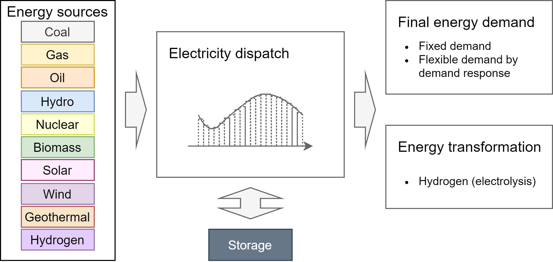
In the power sector, several primary and secondary energy sources, including fossil fuels, nuclear, renewables and hydrogen, are converted to electricity. This sector uses a dispatch module with 1-hour temporal resolution. Four representative days are assessed based on a combination of season (summer, winter) and peak load (peak, off-peak).

Model structure in the power sector

An overview of the technical flow of the power dispatch module is presented below.

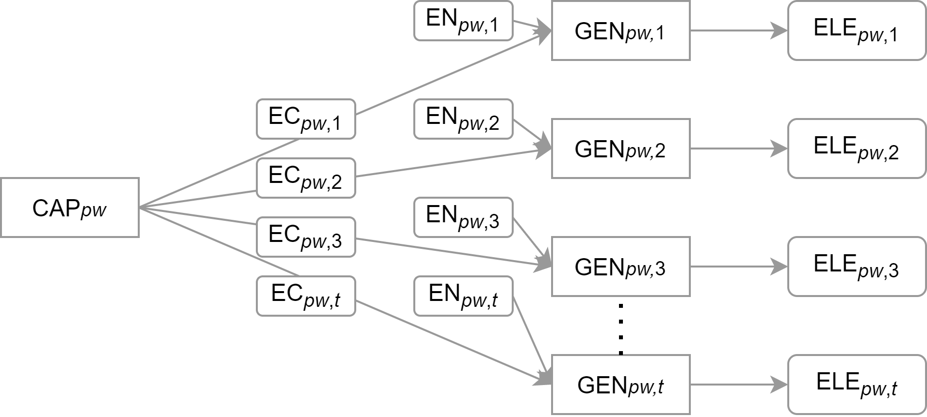
Schematic diagram of the power dispatch module of AIM/Technology. Rectangles indicate devices. Rounded-corner rectangles indicate carriers. The indices pw and ts denote the type of generator (coal, solar, etc.) and time step, respectively.

As shown in the figure, this module is composed of multiple devices and carriers, whereas typical energy technologies are represented with one device and input/output carriers. First, a device “CAP” has the capacity to provide electricity, which is depicted with rounded-corner rectangles labeled “C” for each time step \(t\). The initial cost of power plants is imposed in this device. For electricity capacity devices, the equation on service demand estimation can be rewritten as below (\(\phi_{r,i,l,j}\) is usually zero for electricity capacity devices), with \(a^{cap}\) representing the hourly output profile for VREs, which is set to 1 for other generators.

\[VD_{r,i,j} = \sum_l\{ a^{cap}_{r,i,l,j}\cdot VX_{r,i,l}\},\quad \left(\forall l\in CAP\subset L,\quad j\in EC_{ts}\subset J \right)\]

Second, a device “GEN” provides electricity in each time step, which is represented as “ELE”, given the capacity provided by “CAP” and energy carrier inputs. For flexible generators, such as fossil fuel-burning power plants, the coefficient of output “C” for device “CAP” is constant and is set to 1 across all time steps, while the output “ELE” varies among time steps. For electricity generation devices, equations at each time step can be expressed as below, where e^ene indicates the energy conversion efficiency of power plants, and \(e^{cap}\) and \(e^{ele}\) are both equal to 1. The total amount of power generation is constrained by technology-specific capacity factors. Meanwhile, for variable generators, such as solar PV and wind power, the coefficients are generally less than one and equivalent to the output of the generator. For example, the coefficient of solar PV is set to zero after sunset. The relationship between ELE and EN are defined based on the efficiency parameters of each generator.

\[ \begin{align}\begin{aligned}VE_{r,i,k} = \sum_l\{ e^{ene}_{r,i,l,k}\cdot VX_{r,i,l}\},\quad \left(\forall l\in GEN\subset L,\quad j\in EN_{ts}\subset K \right)\\VE_{r,i,k} = \sum_l\{ e^{cap}_{r,i,l,k}\cdot VX_{r,i,l}\},\quad \left(\forall l\in GEN\subset L,\quad j\in EC_{ts}\subset K \right)\\VD_{r,i,j} = \sum_l\{ a^{ele}_{r,i,l,j}\cdot VX_{r,i,l}\},\quad \left(\forall l\in GEN\subset L,\quad j\in ELE_{ts}\subset J \right)\end{aligned}\end{align} \]

Where, \(CAP\) and \(GEN\) are sets of devices for electricity capacity supply and generation, respectively. \(EC_{ts}\) is a set of dummy carriers representing electricity capacity at each time step. \(EN_{ts}\) and \(ELE_{ts}\) denote carriers for energy input and electricity output, respectively.

The shape of the hourly electricity demand curve is assumed based on the PLEXOS-World dataset [4]. The hourly load curve is affected by demand response using flexible end-use resources, such as electric vehicles and heat-pump water heaters. The technological parameter assumptions of each power plant are based on the literature [5], as summarized in the appendix. Existing power plant data, including capacity, fuel type, and operation start year, are based on the Platts database [6] and the DOE Global Energy Storage Database [7]. Hydro and geothermal potentials were obtained from GEA [8]. Nuclear capacity constraints are from the World Energy Outlook (WEO) and the Energy Technology Perspectives (ETP) [9] [10]. Regarding electricity storage, battery and daily pumped hydro electricity storage (PHES) are modelled for daily storage, and seasonal PHES and compressed air electricity storage for seasonal storage. The potential of PHES and CAES was estimated by the literatures [11] [12].

Hydrogen-based energy production

AIM/Technology models several hydrogen-based energies as secondary energy carriers, including hydrogen, ammonia and synthetic hydrocarbons. Synthetic hydrocarbons include synthetic liquid fuels and synthetic methane. The production method is assumed to be Fischer-Tropsch and methanation for liquid fuels and gases, respectively. Hydrogen can be converted from coal, natural gas, biomass and electricity, and fossil fuels and biomass can be equipped with CCS. The efficiency and cost parameters are based on IEA [13], as summarized in the appendix.

Fossil fuel extraction and production

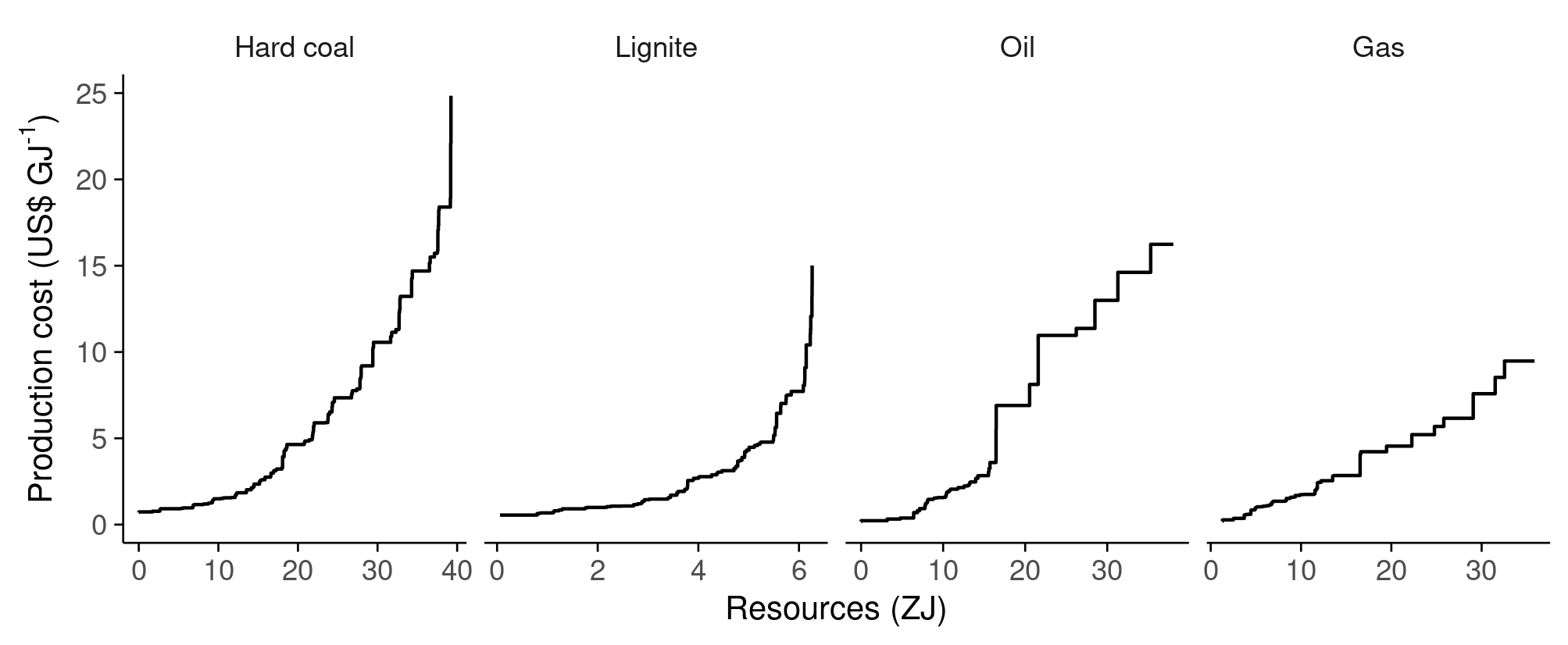
AIM-Technology considers extraction processes for fossil fuels including coal (hard coal, lignite), crude oil and natural gas. The resource potential of each fossil fuel is disaggregated into twelve grades in terms of resource type and extraction cost. Coal reserves and resources are estimated based on the BGR [14]. Extraction cost is based on IIASA-GEA [15], and Bauer et al. [16] [17]. Oil and gas reserves and resources are estimated based on the USGS [18] [19] and BGR [14]. Extraction cost is based on the several literatures [20] [21] [22] . The resource curve for global fossil fuel extraction is shown below.

Resource curve for fossil fuel extraction. Oil includes NGL.

Bioenergy production and conversion

The energy potential of dedicated energy crops is classified into eight grades according to production costs, which are based on the estimates from AIM/PLUM [23] [24]. Other bioenergy including agriculture residue, forest residue, municipal solid waste and manure were obtained from GEA [8]. The bioenergy potential in 2050 is summarized below.

Bioenergy supply potential in 2050. The potential that can be supplied for less than 20 US$ GJ^-1is shown.

Energy sources	Annual energy supply potential (EJ yr-1)
Dedicated energy crops	99.5
Agriculture residue	49.4
Forest residue	35.4
Municipal solid waste	11.0
Manure	39.2

Solar and wind power

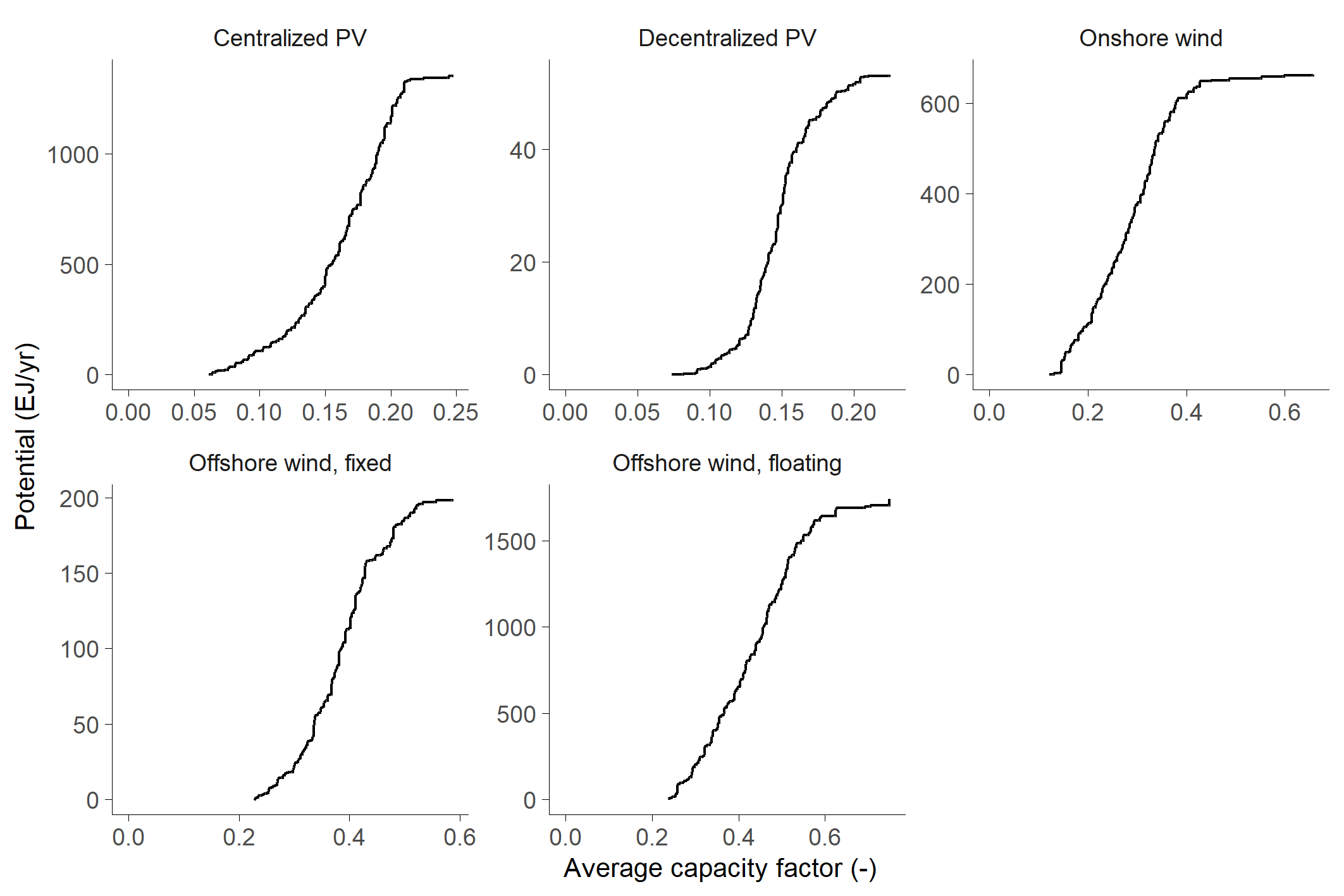
Wind and solar potential and their hourly generation profile are estimated based on climate, weather and land information in 0.5° x 0.5° grid cells. In terms of climate conditions, solar irradiance and wind speed data is taken from MERRA-2 reanalysis data in 2010 [25] [26]. The climate data is converted to hourly power output and physical potential of solar and wind power, based on the formulation and parameter settings of Staffel et al. and Pfenninger et al. [27] [28]. The potentials for solar and wind power is also estimated by suitable land areas, which are summarized as below. Low energy density areas are excluded from the total potential estimation, where annual average wind speed is less than 4.5 and 5.5 m s^-1for onshore and offshore wind, respectively, and annual average capacity factor is less than 5% for solar PV. Finally, solar and wind potentials are classified into eight grade in each region with the level of capacity factor. Total annual solar and wind power potential in 2050 is summarized in the appendix.

Wind and centralized solar PV

For wind power and centralized solar PV, IGBP land cover data [29] is used to estimate the suitable areas and technical potential. Suitable areas for solar and onshore wind power generation is calculated by land suitability factor, which is based on the literatures [30] [31], as summarized in the appendix. Suitability factor for offshore wind is assumed 5%, 40% and 80% of ocean area for the ranges 0-10km, 10-50km and 50-200km from the shore, respectively [31]. Wind turbine capacity density and solar PV panel efficiency are assumed 7MW km^-2and 16%, respectively. For offshore wind, non-EEZ area and distance over 200km from shore area excluded. EEZ area data is taken from the literature [32]. Also, the area with bathymetry more than 50m is classified into floating offshore wind areas. For both solar and onshore/offshore wind power, the protected areas, which are categorized in the IUCN category I-VI, are excluded based on the WDPA [33].

Decentralized solar PV

For decentralized solar PV, potentials in residential area is estimated based on population and household consumption [34], using AIM/Hub [35] and AIM/DS [36] data. Potential in non-residential area is estimated based on area per capita taken from Deng et al. [31].

Wind and solar power generation potential as function of capacity factor

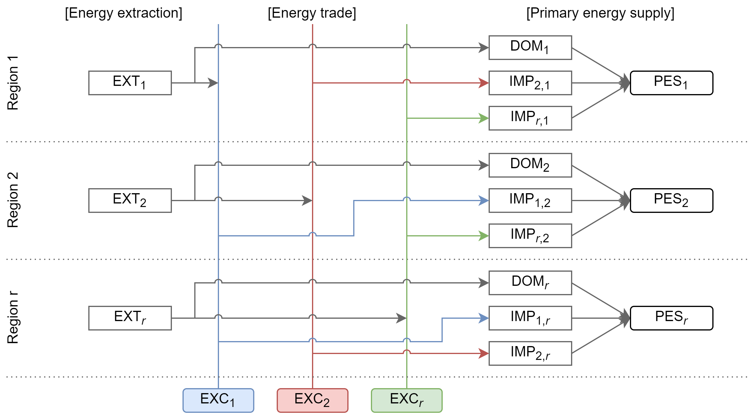
Transport of energy carriers and interregional energy trade

AIM/Technology explicitly considers bilateral trade in coal, crude oil, natural gas, oil products, bioenergy and hydrogen-based fuels (ammonia and synfuels). While all energy carriers are transported primarily by ship, natural gas and crude oil can also be traded by pipeline where currently available. The initial investment and operating costs for energy transport facilities are summarized in the table below based on the literature [37] [38]. A schematic overview of the energy trade flows in AIM/Technology is shown below. EXC and PES represent energy carriers used for interregional trade and primary domestic energy supply, respectively. DOM and IMP indicate domestic energy supply and imports, respectively.

Schematic diagram of interregional energy trade. Rectangles indicate devices. Rounded-corner rectangles indicate carriers. Index \(r\) denotes the region.

Technical parameters for international transport facilities

	Initial investment	O&M costs	Lifetime
	(million US$/GJ)	(US$/GJ*1000km)	(year)
Oil tanker	6.4	0.023	30
LNG tanker	10.2	0.08	20
Bulk ship	2.2	0.014	20
Pipeline	2.0	0.8	30

Carbon capture and sequestration

Carbon capture from large emission sources and direct air capture (DAC) is modeled. CCS from large emission sources includes power and hydrogen generation, oil refineries, bioenergy liquefaction, steel, cement production and furnaces. The parameter assumptions for DAC are summarized below, which is assumed to use hydroxide sorbent, based on Realmonte et al. [39]. Heat supply for DAC can be provided by natural gas, biomass or electricity. Annual potential for underground carbon sequestration is based on IEA [5], and is around 11.5 Gt CO2 in 2050.

Parameter assumptions for DAC

Initial investment (US$/t-CO2)	O&M costs (US$/t-CO2)	Energy inputs	Capture rate (-)
1146	42	1.3 GJe/t-CO2 5.3 GJHeat/t-CO2	95%

Historical period calibration

The simulation start year is set to 2005 for this model, and most parts of the energy system between 2005 and 2015, for which historical data are available, are calibrated based on IEA [40]. The installation of energy technology during each period is determined exogenously so that sectoral energy demand and supply meet the corresponding statistical values.

\[\tau_{r,i,l}^{min,y} = r\_h_{r,i,l}^y\]

Where, \(r\_h_{r,i,l}^y\) is the minimum installed capacity of device \(l\) in year \(y\) for historical data calibration.

Energy service demand

Energy service demand is estimated based on Akashi et al. [41] [2]. Economic growth and population growth are the fundamental drivers of demand, and their assumptions are determined exogenously based on representative scenarios such as Shared Socio-economic Pathways (SSPs) [42]. The energy service indicators used for each sector are summarized below. The industrial sector includes various service demands for crude steel and cement production, while useful energy includes fuel for heat, motors and other uses. In the buildings sector, energy service demand is classified into several energy services, including space heating and cooling, water heating, cooking, lighting and appliances in the residential and commercial sectors. Energy service demand for the transport sector is presented for multiple modes, namely road, rail, maritime navigation and aviation for both passenger and freight. The basic structure, equations, and parameters were reported in Akashi et al. [41] [2]. Historical socio-economic indicators, such as GDP and population, are based on the World Development Indicators [43].

List of energy service indicators in each sector

Sector		Energy service indicator
Industry	Steel	Crude steel production
	Cement	Cement production
	Other	Useful energy for heating, electronics and other purposes
Buildings	Residential / Commercial	Useful energy for space heating/cooling, water heating, cooking, lighting and other appliances
Transport	Passenger / Freight	Transport demand for road, rail, maritime and aviation transport. Domestic and international transport are separated for navigation and aviation

Industry

Industrial service demand estimation is based on the method of Akashi et al. [41]. Crude steel production is estimated using a global steel demand and production model developed by [41]. The domestic and international market equilibrium equations are presented as equations below.

\[CNS_r = PRD_r - EXC_r + MC_r\]

\[\sum_r EXC_r = \sum_r MC_r\]

Cement production per capita is estimated through semi-log linear regression using the natural logarithm of GDP-PPP per capita as an explanatory variable. The regression results are summarized in the appendices.

\[PRDP_{r,t}^{cem} = \alpha^{cem} + \beta^{cem}\cdot \ln{GDPP_{r,t}^*} + \gamma_r^{cem}\cdot DUM_r\]

In the other industry sector, energy service demand is estimated with a log-log function. The regression results are summarized in the appendices.

\[SRVP_{r,t}^{oin} = \exp\left(\alpha^{oin} + \beta^{oin}\cdot \ln{VA\_INDP_{r,t}^*} + \gamma_r^{oin}\cdot DUM_r \right)\]

Where \(PRDP_{r,t}^{cem}\) and \(SRVP_{r,t}^{oin}\) are cement production and other industry service demand per capita in region \(r\), respectively. \(GDPP_{r,t}^*\) and \(VA\_INDP_{r,t}^*\) represent GDP-PPP per capita and industry value-added per capita, respectively. \(DUM_r\) is a dummy variable for region \(r\).

Transport

Transport demand estimation in AIM/Technology is based on Akashi et al. [44]. First, total passenger transport demand per capita is estimated with a log-log function using GDP-PPP per capita as an explanatory variable. The parameters (\(\alpha^{pk}, \beta^{pk}, \gamma^{pk}\)) are determined through the least squares method, and their regression results are summarized in appendices.

\[PKTOTP_{r,t} = \exp\left(\alpha^{pk}+\beta^{pk}\cdot\ln GDPP_{r,t}^*+\gamma_r^{pk}\cdot DUM_r\right)\]

Second, the modal share is estimated with a multinomial logit model using GDP-PPP per capita as an explanatory variable. The regression results are summarized in appendices.

\[PKSH_{r,m,t} = \frac{\exp\left(\alpha_m^{pksh}+\beta_m^{pksh}\cdot\ln GDPP_{r,t}^*+\gamma_{r,m}^{pksh}\cdot DUM_r \right)}{\sum_m \exp\left(\alpha_m^{pksh}+\beta_m^{pksh}\cdot \ln GDPP_{r,t}^*+\gamma_{r,m}^{pksh}\cdot DUM_r \right)},\quad \forall m\in {PK}\]

where \(PKTOTP_{r,t}\) is total passenger transport demand per capita in region \(r\). \(GDPP_{r,t}^*\) represents GDP-PPP per capita. \(DUM_r\) is dummy variable for region \(r\). \(PKSH_{r,m,t}\) is model share of passenger transport. \(PK\) includes the mode options in the passenger transport sector.

Freight transport demands for road and rail are estimated in a manner identical to that of passenger transport. The total freight passenger demand in road and rail is estimated by log-log function as shown below. The regression result is provided in appendices.

\[TKTOTP_{r,t} = \exp\left(\alpha^{tk}+\beta^{tk}\cdot\ln GDPP_{r,t}^*+\gamma_r^{tk}\cdot DUM_r\right)\]

Modal share between road and rail is estimated by logit function as shown below, with the regression result in appendices.

\[TKSH_{r,m,t} = \frac{\exp\left(\alpha_m^{tksh}+\beta_m^{tksh}\cdot\ln GDPP_{r,t}^* +\gamma_{r,m}^{tksh}\cdot DUM_r \right)}{\sum_m \exp\left(\alpha_m^{tksh}+\beta_m^{tksh}\cdot\ln GDPP_{r,t}^*+\gamma_{r,m}^{tksh}\cdot DUM_r\right)},\quad \forall m\in TK\]

Freight transport demand by navigation is estimated separately from other modes, using a natural logarithm of GDP-PPP as an explanatory variable with a region dummy. The regression results are summarized in appendices.

\[TKN_{r,m,t} = \exp\left(\alpha_m^{tkn}+\beta_m^{tkn}\cdot \ln GDP_{r,t}^*+\gamma_{r,m}^{tkn}\cdot DUM_r\right),\quad \forall m\in TKN\]

where \(TKTOTP_{r,t}\) is total passenger transport demand in region \(r\). \(TKSH_{r,m,t}\) is the modeled share of passenger transport. \(TK\) includes road and rail transport. \(TKN_{r,m,t}\) is freight transport demand for navigation. \(TK\) includes maritime navigation for domestic and international transport.

Buildings

Residential and commercial service demands are estimated based on the several drivers using a log-log function weighted by population size. Total service demand for cooking is estimated from population size. The regression results are summarized in appendices. Historical data on energy consumption were obtained from IEA [45].

\[RSTOTP_{r,rs,t} = \exp\left(\alpha_{rs}^{rsd}+\beta_{rs}^{rsd}\cdot\ln GDPP_{r,t}^*+\gamma_{r,rs}^{rsd}\cdot DUM_r+\delta_{rs}^{rsd}\cdot\ln HDD_{r,t}+\epsilon_{rs}^{rsd}\cdot\ln CDD_{r,t}\right)\]

\[RSTOTP_{r,"RHW",t} = \exp\left(\alpha_{rs}^{rsd}+\beta_{rs}^{rsd}\cdot\ln GDPP_{r,t}^*+\gamma_{r,rs}^{rsd}\cdot DUM_r+\delta_{rs}^{rsd}\cdot HDD_{r,t}\right)\]

\[RSTOT_{r,"RCK",t} = \exp\left(\alpha_{"RCK"}^{rsd}+\beta_{"RCK"}^{rsd}\cdot\ln POP_{r,t}+\gamma_{r,"RCK"}^{rsd}\cdot DUM_r\right)\]

\[RSTOT_{r,rs,t} = POP_{r,t}\cdot RSTOTP_{r,rs,t}\]

where \(RSTOTP_{r,rs,t}\) is residential service demand per capita for service \(rs\) in region \(r\). \(HDD_{r,t}\) and \(CDD_{r,t}\) represent heating and cooling degree days, respectively.

\[SRTOTP_{r,ss,t} = \exp\left(\alpha_{ss}^{ser}+\beta_{ss}^{ser}\cdot\ln GDPP_{r,t}^*+\gamma_{r,ss}^{ser}\cdot DUM_r+\delta_{ss}^{ser}\cdot \ln HDD_{r,t}+\epsilon_{ss}^{ser}\cdot\ln CDD_{r,t}\right)\]

\[SRTOT_{r,ss,t} = POP_{r,t}\cdot SRTOTP_{r,ss,t}\]

where \(SRTOTP_{r,ss,t}\) is commercial service demand per capita for service ss in region \(r\).

Drivers used for estimating energy service demand in the buildings sector

Sector	Energy service	Driver
Residential	Space heating	GDP per capita, Heating degree days (HDD)
	Space cooling	GDP per capita, Cooling degree days (CDD)
	Water heating	GDP per capita
	Cooking	Population
	Lighting and other appliances	GDP per capita
Commercial	Space heating	GDP per capita, HDD
	Space cooling	GDP per capita, CDD
	Other services	GDP per capita

References

[1]	(1, 2) USDOE. (2003). Model Documentation Report: System for the Analysis of Global Energy Markets (SAGE) - Vol. II, Model Documentation. https://www.eia.gov/analysis/pdfpages/m072(2003)2index.php

[2]

(1, 2, 3) Akashi, O., Ashina, S., Ehara, T., Fujino, J., Fujiwara, T., Hanaoka, T., Hanasaki, N., Harasawa, H., Hibino, G., Hijioka, Y., Kainuma, M., Kawase, R., Masui, T., Matsuoka, Y., Miyashita, M., Shimada, K., Shukla, P. R., Takahashi, K. (2007). Aligning Climate Change and Sustainability -Scenarios, modeling and policy analysis-. https://www.cger.nies.go.jp/publications/report/i072/I072.pdf

[3]	Akashi, O., Hijioka, Y., Masui, T., Hanaoka, T., Kainuma, M. (2012). GHG emission scenarios in Asia and the world: The key technologies for significant reduction. Energy Economics, 34, S346-S358. https://doi.org/10.1016/j.eneco.2012.04.011

[4]	Brinkerink, M., Deane, P. (2020). PLEXOS-World 2015. https://doi.org/10.7910/DVN/CBYXBY

[5]	(1, 2) IEA. (2018). World Energy Outlook 2018. Paris: OECD/IEA.

[6]	Platts. (2014). World Electric Power Plants Database.

[7]	USDOE. (2021). DOE Global Energy Storage Database. Retrieved from: https://sandia.gov/ess-ssl/gesdb/public/

[8]	(1, 2) GEA. (2012). Global Energy Assessment - Toward a Sustainable Future. Cambridge University Press, Cambridge, UK and New York, NY, USA and the International Institute for Applied Systems Analysis, Laxenburg, Austria.

[9]	IEA. (2019). World Energy Outlook 2019. Paris: OECD/IEA.

[10]	IEA. (2017). Energy Technology Perspectives 2017. Paris: OECD/IEA.

[11]	Aghahosseini, A., Breyer, C. (2018). Assessment of geological resource potential for compressed air energy storage in global electricity supply. Energy Conversion and Management, 169, 161-173. https://doi.org/10.1016/j.enconman.2018.05.058

[12]	Stocks, M., Stocks, R., Lu, B., Cheng, C., Blakers, A. (2021). Global Atlas of Closed-Loop Pumped Hydro Energy Storage. Joule, 5(1), 270-284. https://doi.org/10.1016/j.joule.2020.11.015

[13]	IEA. (2019). The Future of Hydrogen Seizing today’s opportunities. https://www.iea.org/reports/the-future-of-hydrogen

[14]	(1, 2) BGR. (2009). Energy Resources 2009 - Reserves, Resources, Availability - Crude Oil, Natural Gas, Coal, Nuclear Fuels, Geothermal Energy.

[15]

Rogner, H.-H., Aguilera, R. F., Archer, C., Bertani, R., Bhattacharya, S. C., Dusseault, M. B., Gagnon, L., Haberl, H., Hoogwijk, M., Johnson, A., Rogner, M. L., Wagner, H., Yakushev, V. (2012). Chapter 7 - Energy Resources and Potentials. In Global Energy Assessment - Toward a Sustainable Future (pp. 423-512). Cambridge University Press, Cambridge, UK and New York, NY, USA and the International Institute for Applied Systems Analysis, Laxenburg, Austria.

[16]	Bauer, N., Hilaire, J., Brecha, R. J., Edmonds, J., Jiang, K., Kriegler, E., Rogner, H.-H., Sferra, F. (2016). Assessing global fossil fuel availability in a scenario framework. Energy, 111, 580-592. https://doi.org/10.1016/j.energy.2016.05.088

[17]	Bauer, N., Hilaire, J., Brecha, R. J., Edmonds, J., Jiang, K., Kriegler, E., Rogner, H.-H., Sferra, F. (2017). Data on fossil fuel availability for Shared Socioeconomic Pathways. Data in Brief, 10, 44-46. https://doi.org/10.1016/j.dib.2016.11.043

[18]	USGS. (2000). U.S. Geological Survey world petroleum assessment 2000: Description and results (60). https://pubs.usgs.gov/publication/ds60

[19]	USGS. (1995). USGS. (1995). 1995 National Assessment of United States Oil and Gas Resources. https://pubs.usgs.gov/circ/1995/1118/report.pdf

[20]	Aguilera, R. F., Eggert, R. G., Gustavo Lagos, C. C., Tilton, J. E. (2009). Depletion and the Future Availability of Petroleum Resources. The Energy Journal, 30(1), 141-174. https://doi.org/10.5547/ISSN0195-6574-EJ-Vol30-No1-6

[21]	Rogner, H.-H. (1997). An assessment of world hydrocarbon resources. Annual Review of Energy and the Environment, 22(1), 217-262. https://www.annualreviews.org/doi/abs/10.1146/annurev.energy.22.1.217

[22]	IEA. (2013). Resources to Reserves 2013: Oil, Gas and Coal Technologies for the Energy Markets of the Future. Paris: International Energy Agency.

[23]	Hasegawa, T., Fujimori, S., Ito, A., Takahashi, K., Masui, T. (2017). Global land-use allocation model linked to an integrated assessment model. Science of The Total Environment, 580, 787-796. https://doi.org/10.1016/j.scitotenv.2016.12.025

[24]

Wu, W., Hasegawa, T., Ohashi, H., Hanasaki, N., Liu, J., Matsui, T., Fujimori, S., Masui, T., Takahashi, K. (2019). Global advanced bioenergy potential under environmental protection policies and societal transformation measures. GCB Bioenergy, 11(9), 1041-1055. https://onlinelibrary.wiley.com/doi/abs/10.1111/gcbb.12614

[25]	Global Modeling and Assimilation Office (GMAO). (2015). MERRA-2 tavg1_2d_rad_Nx: 2d,1-Hourly,Time-Averaged,Single-Level,Assimilation,Radiation Diagnostics V5.12.4.

[26]	Global Modeling and Assimilation Office (GMAO). (2015). MERRA-2 tavg1_2d_slv_Nx: 2d,1-Hourly,Time-Averaged,Single-Level,Assimilation,Single-Level Diagnostics V5.12.4.

[27]	Staffell, I., Pfenninger, S. (2016). Using bias-corrected reanalysis to simulate current and future wind power output. Energy, 114, 1224-1239. https://doi.org/10.1016/j.energy.2016.08.068

[28]	Pfenninger, S., Staffell, I. (2016). Long-term patterns of European PV output using 30 years of validated hourly reanalysis and satellite data. Energy, 114, 1251-1265. https://doi.org/10.1016/j.energy.2016.08.060

[29]	Friedl, M. A., Sulla-Menashe, D. (2015). MCD12C1 MODIS/Terra+Aqua Land Cover Type Yearly L3 Global 0.05Deg CMG V006. https://doi.org/10.5067/MODIS/MCD12C1.006

[30]	Hoogwijk, M. (2004). On the global and regional potential of renewable energy sources. Utrecht University, Utrecht. https://dspace.library.uu.nl/handle/1874/782

[31]	(1, 2, 3) Deng, Y. Y., Haigh, M., Pouwels, W., Ramaekers, L., Brandsma, R., Schimschar, S., Grözinger, J., de Jager, D. (2015). Quantifying a realistic, worldwide wind and solar electricity supply. Global Environmental Change, 31, 239-252. doi:10.1016/j.gloenvcha.2015.01.005

[32]	Flanders Marine Institute. (2019). Maritime Boundaries Geodatabase: Maritime Boundaries and Exclusive Economic Zones (200NM), version 11. https://www.marineregions.org/

[33]	UNEP-WCMC, IUCN. (2019). The World Database on Protected Areas (WDPA)/OECM Database. https://www.protectedplanet.net/

[34]	Gernaat, D. E. H. J., de Boer, H.-S., Dammeier, L. C., van Vuuren, D. P. (2020). The role of residential rooftop photovoltaic in long-term energy and climate scenarios. Applied Energy, 279, 115705. doi:10.1016/j.apenergy.2020.115705

[35]	Fujimori, S., Hasegawa, T., Masui, T., Takahashi, K., Herran, D. S., Dai, H., Hijioka, Y., Kainuma, M. (2017). SSP3: AIM implementation of Shared Socioeconomic Pathways. Global Environmental Change, 42, 268-283. doi:10.1016/j.gloenvcha.2016.06.009

[36]	Fujimori, S., Hasegawa, T., Ito, A., Takahashi, K., Masui, T. (2018). Gridded emissions and land-use data for 2005–2100 under diverse socioeconomic and climate mitigation scenarios. Scientific Data, 5(1), 180210. doi:10.1038/sdata.2018.210

[37]	IEA-ETSAP. (2011). IEA-ETSAP Technology brief. https://iea-etsap.org/index.php/energy-technology-data

[38]	Bauer, N., Mouratiadou, I., Luderer, G., Baumstark, L., Brecha, R. J., Edenhofer, O., Kriegler, E. (2016). Global fossil energy markets and climate change mitigation – an analysis with REMIND. Climatic Change, 136(1), 69-82. https://doi.org/10.1007/s10584-013-0901-6

[39]	Realmonte, G., Drouet, L., Gambhir, A., Glynn, J., Hawkes, A., Köberle, A. C., Tavoni, M. (2019). An inter-model assessment of the role of direct air capture in deep mitigation pathways. Nature Communications, 10(1), 3277. https://doi.org/10.1038/s41467-019-10842-5

[40]	IEA. (2018). World Energy Balances. Paris: OECD/IEA.

[41]	(1, 2, 3, 4) Akashi, O., Hanaoka, T., Matsuoka, Y., Kainuma, M. (2011). A projection for global CO2 emissions from the industrial sector through 2030 based on activity level and technology changes. Energy, 36(4), 1855-1867. https://doi.org/10.1016/j.energy.2010.08.016

[42]

Riahi, K., van Vuuren, D. P., Kriegler, E., Edmonds, J., O’Neill, B. C., Fujimori, S., Bauer, N., Calvin, K., Dellink, R., Fricko, O., Lutz, W., Popp, A., Cuaresma, J. C., Kc, S., Leimbach, M., Jiang, L., Kram, T., Rao, S., Emmerling, J., Ebi, K., Hasegawa, T., Havlik, P., Humpenöder, F., Da Silva, L. A., Smith, S., Stehfest, E., Bosetti, V., Eom, J., Gernaat, D., Masui, T., Rogelj, J., Strefler, J., Drouet, L., Krey, V., Luderer, G., Harmsen, M., Takahashi, K., Baumstark, L., Doelman, J. C., Kainuma, M., Klimont, Z., Marangoni, G., Lotze-Campen, H., Obersteiner, M., Tabeau, A., Tavoni, M. (2017). The Shared Socioeconomic Pathways and their energy, land use, and greenhouse gas emissions implications: An overview. Global Environmental Change, 42, 153-168. https://doi.org/10.1016/j.gloenvcha.2016.05.009

[43]	The World Bank. (2019). World Development Indicators. Retrieved from https://databank.worldbank.org/source/world-development-indicators

[44]	Akashi, O., Hanaoka, T., Masui, T., Kainuma, M. (2014). Halving global GHG emissions by 2050 without depending on nuclear and CCS. Climatic Change, 123(3), 611-622. https://doi.org/10.1007/s10584-013-0942-x

[45]	IEA. (2019). Energy efficiency indicators. Paris: OECD/IEA.